DC2DInvRes - Model Menu

Model parameter

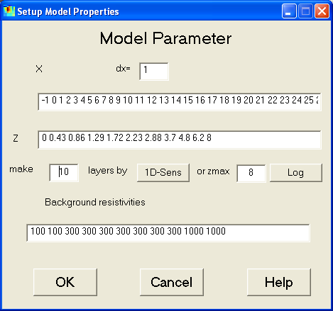
This dialog is used to control the model parameterizations.

By typing dx a new (equidistant) x-grid is defined, which also can be edited manually.
The boundaries of the model layers can be changed both manually or automatically (by regarding 1D sensitivities or by constructing logarithmically increasing thicknesses for a given model depth).
Furthermore, the background resistivities can be set up. In the presented example a three-layer case is introduced. Note, that the number of Background resistivities must equal the number of z-Layers, since the last resistivity is that below the model.

Pick Cell

Now you can click on any cell in order to show cell dimensions, resistivity and ip phase (if present).
Note that this is done by setting the resistivity window to 0 or empty it.

Homogeneous model

This resets all model cells (and background resistivities) back to the homogeneous half-space of the median resistivity.

Hotkey: Shift+H

Export model

For further work or manual plots the model can be exported into an column-oriented model file (*.mod) of the following format:

x_1 x_2 z_1 z_2 resistivity (coverage)
...

The model files can be used for postprocessing as well as for saving purposes. It is recommended to save important inversion models as model file. Thus it is possible to print the model at a later time.

Import model

The exported model is loaded from ASCII type model file (*.mod) into workspace. It may be a synthetic model, a starting/reference model or a formerly save inversion result.

Compare models

For several reasons like synthetic model studies, it might be useful to determine the distance of two models.
After clicking, a input file dialog opens to select a model file (*.mod) on disk. The rms error between the current model and the model on disk is diplayed in a dialog.

Cluster analysis

Often we wish to obtain a simplified model concept. This might be accomplished by means of a cluster analysis. Besides the resistivity (and ip phase if present) the geometrical position, i.e. x and z of the midpoint, is included to result in more compact models.
We use euclidean distances and complete linkage for the hierarchical seperation. After this we show the cluster function (cluster number vs. total distance) and the user is asked to specify the cluster number. If not determined by geology or visual, we often search a L-shaped corner as for the selection of regularization parameter.
Then the median value of each cluster is associated to all its members.